
Introduction
The interplay between the mathematics and the sciences is always an interesting one to explore, and the current COVID-19 pandemic presents an opportunity to apply some of that pure mathematics in a real world context. This project will attempt to explore and demonstrate how these models could be applied to real-world data on the epidemic trajectory in several different countries.
The 2020 COVID-19 pandemic is the result of a viral disease, SARS-CoV-2, that had originated in Wuhan, China that spread globally in a period of less than 3 months. Different mathematical models could be applied to describe this event, and the aim of this research investigation is the focus on how one such mode, the S-I-R model, could be used. This investigation will follow 3 main parts:
- I will explain how the set of differential equations describing the S-I-R model could be turned into an iterative relation. This could then be turned into a Python program which is attached in the Appendices.
- I will vary the values of the parameters, specifically, the initial number of cases, the transmission rate and the recovery rate (which will be defined later) and assess their impact on the hypothetical progression of an unchecked COVID-19 pandemic in Singapore. These values are cited from the latest published research as of April, 2020.
- I will assess the impact of government controls placed on the COVID-19 spread and compare that with what different countries have implemented.
The report is part of a school project completed during the COVID-19 pandemic intended to raise awareness and interest within the school community about the applicability of mathematics to the real world.
Background Information
There are a whole host of different mathematical models that could be used to describe the growth and development of an epidemic, but they can mostly be classified into phenomenological and mechanistic models.
| Phenomenological Model | Exponential Regression Logistic Regression |
| Mechanistic Model | S-I-R Model S-E-I-R Model Other Computer Simulations |
Examples of phenomenological and mechanistic models.
Phenomenological models use equations such as exponential and logistic functions for regression analysis of real epidemiological data. However, this process suffers several drawbacks. Exponential functions are only valid for modelling the initial stages of the outbreak. Even logistic functions are not perfect, as they are often dependent upon reliable data, which is contingent upon efforts made by the respective national governments. Both models have weak predictive power and generalisability, as they rely on “curve fitting” to real-world data rather than based upon an underlying natural mechanism. Innate characteristics of a disease, such as transmissibility and recovery rate, are not accounted for in this model.
The first real breakthrough in the development of further epidemiological models and paved the way for further progress is the Susceptible-Infectious-Removed (S-I-R) mechanistic model. Mechanistic models are based upon the quantifiable characteristics of the disease. The model, developed by Kermack and McKendrick in 1927, is a set of 3 differential equations that describe how 3 groups of individuals change over time based upon 2 key parameters.
The 3 groups are:
- S: Susceptible cases– The number of cases in a population that would be at risk of an infection. For a completely novel pathogen, such as SARS-CoV-2, it may be assumed that the entire population (of a country, for example) is susceptible.
- I: Infectious cases– The number of cases in a population that are currently infectious and are actively spreading disease.
- R: Removed cases– Removed (sometimes called recovered even though it is the sum of recovered and dead) cases are cases that have either recovered and gained immunity or have passed away (and thus will not become susceptibles again).
Incidentally, this is where the name of the model comes from.
The 2 parameters are:
- Duration of disease,
, is the number of days that a person is infectious since the beginning of the disease. It is assumed that a person is immediately infectious since they are first infected.
- Basic Reproductive Number,
, characterizes the average number of new cases that would become infected by 1 infectious case over the entire duration of his disease. It is generally fixed in the beginning of a disease.
Let’s assume a certain disease has an  , and , and  , and , and  person in a population of person in a population of  gets it. gets it. , as person already has the disease. , as person already has the disease.On each day the person is infectious, he or she will infect on average  new individuals per day, this is called the “rate of infection”. If we assume that everyone in the population has an equal chance of getting the disease (a key assumption of the S-I-R model), then the probability of me, a random person, getting the disease at the on the first day will be new individuals per day, this is called the “rate of infection”. If we assume that everyone in the population has an equal chance of getting the disease (a key assumption of the S-I-R model), then the probability of me, a random person, getting the disease at the on the first day will be  . .Epidemiologists call this the “force of infection,” denoted as . The force of infection is not fixed, and it is clear that the larger the population, given the same , the lower the probability that any one individual would become infected. The force of infection is important for establishing the S-I-R Model.Another important quantity is the “rate of recovery”, denoted as . As it takes D days for an infected person to recover, infected people recover at a rate equal to the reciprocal, so  . . |
The 3 differential equations first proposed by Kermack and McKendrick in 1927 were:


There are a several important things to unpack:
- The rate of new infections is directly proportional to the number of people infected, and the number of people susceptible. So as the susceptible population decreases as they become infected, the rate of new infections decreases.
- The rate of change of infections equals the rate of new recoveries subtracted from the rate of new infections. Thus, the peak of infections occurs when
.
- The rate of new recoveries is directly proportional the the number of people currently infected, as the more infected people their are, the greater recoveries per unit time there are.
Project Timeline Log
| Tasks | Comments |
| Essential Background Research, Create Annotated Reference List
(March 3rd to April 11th) |
|
| Developed and Focused Research Questions
(April 12th to April 19th) |
|
| Programmed essential programs in Python with MatPlotLib library
(April 20th to April 28th) |
|
| Analysis and Interpretation of of Results, Creating graphs in Python, Write up into Project Report and proofing
(April 26th to May 6th) |
|
| Project Finalization and Sharing with Peers and School Audience |
|
Creating the Initial S.I.R. Model in Python
The system of differential equations is difficult to solve analytically, and as mentioned previously, I will convert this into a Python program. The model works by iterating the model over many small time intervals.
The recursive relations based on the differential equations are as follows, where 
=S(t)-\beta \cdot S(t) \cdot I(t)")
=I(t)+\beta \cdot S(t) \cdot I(t) - \gamma \cdot I(t)")
=R(t)+\gamma \cdot I(t)")
This article, The S-I-R Model for Spread of Disease, from the Mathematical Association of America, though a bit dated, gives a good general overview of the iteration process.
The initial conditions are first defined:
S=5804000-1
I=1
R=0
R0=2.6
d=10
I used ‘a’ to represent 
I then create 3 lists where the successive values will be appended.
susceptible=[5804000-1]
infected=[1]
recovered=[0]
Using this, a for loop can be created that runs the model over a certain time period, for example 200 days, and the values are appended onto the list each iteration:
for t in range (1,period+1):
S=S-S*I*a
I=I+S*I*a-I/d
R=R+I/d
susceptible.append(S)
infected.append(I)
recovered.append(R)
Using the MatPlotLib library as import matplotlib.pyplot as plt, a graph is created, which is Graph 1.1 in the following section.
plt.plot(time, susceptible, color='b', label='Susceptible')
plt.plot(time, infected, color='r', label='Infected')
plt.plot(time, recovered, color='g', label='Recovered')
plt.xlabel('Time (days)')
plt.ylabel('Number of Individuals')
This part of the code is provided in full in Appendix A.
COVID-19 in Singapore: Hypothetical Unmitigated Scenario
The World Health Organization has estimated that the basic reproductive number, 


According to an analysis done by the National University of Singapore, the mean duration from the onset of symptoms such as fever and cough until the clearance of the virus was 


")
| Singapore Population |  (2019) (2019) |
| Initial Force of Infection () |
 |
Rate of Recovery ( ) ) |
 |
Singapore S-I-R Model Key Characteristics
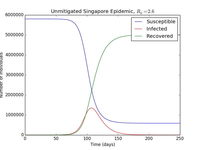 Graph 1.1– Unmitigated Singapore Epidemic,  , ,  |
As can be seen in Graph 1.1, the blue curve and green curve seem to be logistic functions, and at the start of the epidemic, they are similar to exponentials. We can look back at the differential equation that describes the rate of change of susceptible individuals:
In the initial stages of the outbreak, Sstays relatively constant, as the number of infected cases is much small in relation to the entire population, i.e. 

 \cdot I")


 dt")
 dt")
=(r- \gamma )t+c")
t+c}")
t}")
Substituting into 
t}")
t}dt")
t}dt")
t}+S_{0}")

Substituting the values of 


Plotting these two equations with the S-I-R Model yields the following graph.
 Graph 1.2– S-I-R Model v.s. Exponential Model |
As can be seen in Graph 1.2, the exponential model agrees very well for the initial stages of the pandemic, but rapidly diverges after perhaps Day 80 as it does not take herd immunity into account (which decreases the rate of infection).
The equation 


This equation allows for easier analysis and comparison with government available raw data in the Addendum.
Effect of Varying the Reproductive Number,
Varying the
Basic Reproductive Number  |
Peak Proportion of Pop. Infected | Final Epidemic Size | Final Epidemic Size as Proportion of Pop. |
| 1.0 | 0.00% | 51 | 0.00% |
| 1.2 | 1.46% | 112,000 | 1.92% |
| 1.3 | 2.86% | 1,932,172 | 33.3% |
| 1.4 | 4.47% | 2,930,000 | 50.5% |
| 1.6 | 7.95% | 3,700,000 | 63.8% |
| 1.8 | 11.4% | 4,220,000 | 72.8% |
| 2.0 | 14.8% | 4,590,000 | 79.1% |
| 2.2 | 17.9% | 4,860,000 | 83.8% |
| 2.4 | 20.7% | 5,060,000 | 87.3% |
| 2.6 | 23.3% | 5,210,000 | 89.9% |
| 2.8 | 25.6% | 5,330,000 | 91.9% |
| 3.0 | 27.8% | 5,420,000 | 93.5% |
As can be seen even from the data, there are disastrous consequences when no measures are put in place and individuals do nothing to change their behavior. Even with the WHO’s conservative estimate of an
According to the World Health Organization, Singapore has an average of 2.4 hospital beds per 1000 people, or 0.24% of the population. Assuming that 5% of patients required hospitalization, during the peak of the infections for
Using even this basic model, the results are comparable to values determined up by researchers using much more advanced mathematical analysis at Imperial College London. According to a report released on March 3rd, 2020: modelling an unmitigated epidemic in the United Kingdom, for an 

The plot of the peak proportion of the population and the final epidemic size are the graphs below. (see code in Appendix B and Appendix C)
 Graph 1.3– Final Epidemic Size as Proportion of Population Against from  to to  |
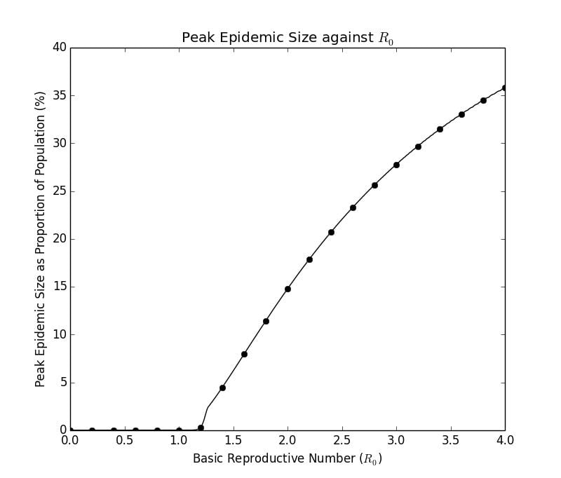 Graph 1.4– Peak Epidemic Size as Proportion of Population Against from to |
It is very difficult to determine the analytical solution for these values of
As can be seen in Graph 1.3, for 


Graph 1.4 indicates the peak proportion of the population that will be infected at one time based upon the
Comparing COVID-19 with seasonal influenza, which according to a meta-analysis done by researchers at the Centers for Disease Control and Prevention, has a median 
This evaluation shows how COVID-19 is much more transmissible and severe than the influenza, and a herd immunity approach is likely going to cause a significant amount of morbidity and mortality. As there is no vaccine available at the current moment, this indicates the disease’s high potential for overwhelming any country’s healthcare system.
Effect of the Varying the Initial Number of Cases, 
Another important effect to consider is the effect of the number of imported coronavirus cases (initial infectious cases, 


 Graph 2.1- Solid line: =1") , Dotted line: , Dotted line: =1000") , ,  , , |
Some representative values for the number of imported cases are chosen. The day of the peak of infectious population, and peak proportion of infections is determined (See code in Appendix D).
To determine the relationship between the relationship between the number of imported cases and the day with the peak number of infections, a plot of the number of imported cases vs the number of days earlier that the outbreak happened as compared with the case when 

| Number of Imported Cases, |
Peak Proportion of Pop. Infected | Day with the Peak number of Infections | Number of Days Earlier, k |
| 1 | 23.29% | 107 | 0 |
| 5 | 23.29% | 96 | 11 |
| 10 | 23.28% | 92 | 15 |
| 50 | 23.29% | 81 | 26 |
| 100 | 23.29% | 76 | 31 |
| 500 | 23.30% | 65 | 42 |
| 1,000 | 23.29% | 61 | 46 |
| 10,000 | 23.41% | 45 | 62 |
In Python, a linear regression was fitted to ")
=0.1490k+0.0150")


=0.1490k+0.0150")

For the purposes of the model fitting,
-0.0150")
-1.007")
 Graph 2.2– Semilog Plot of against , , |
 Graph 2.3– Normal Plot of against , , |
The reason for this is because the spread in the initial stages of an epidemic is very close to an exponential model. Using equation (1) model obtained at the start  . .
+0.16t}=e^{1+\frac{ln(I_0)}{0.16}}\cdot 0.16t=e^{0.16(6.25ln(I_0)+1)t}")
This is equivalent to a horizontal translation of +1")
This is close to |
-1}") from
from 
-1.007") that we have derived from the above.
that we have derived from the above.The result has significant implications for managing an epidemic, as it shows where the benefits of the travel restrictions are the greatest, as well as the reason for the large delay between countries where there is epidemic spread. Although the model is based on Singapore, it could be re-applied to other countries with appropriate population adjustments.
Some representative cities and the day when the cumulative case count surpassed 100 are listed in the chart below. Part of the reason for the latent outbreak as severe or even more severe than Wuhan was due to the frequency of international travel from Wuhan to these cities, which is related to geographic proximity to China.
| People’s Republic of China | South Korea | Italy | UK | USA | ||
| City | Wuhan | Shanghai | Daegu | Lombardy | London | New York |
| Date | Jan. 18th | Jan. 29th | Feb. 21st | Feb. 23rd | March 12th | March 13th |
| Delay | 0 | 11 | 34 | 36 | 54 | 55 |
The effect of travel restrictions could also be explored here.
Assume that the original number of imported cases is ,
-1.007")
If travel restrictions reduce the number of imported cases by 80%,
Thus, the reduction is invariant to the absolute number of cases: whether reducing the number of imported cases from |

-1.007")
![k_{new}=6.711ln(0.2)+[6.711ln(I_0)-1.007]](http://s0.wp.com/latex.php?latex=k_%7Bnew%7D%3D6.711ln%280.2%29%2B%5B6.711ln%28I_0%29-1.007%5D&bg=ffffff&fg=000000&s=0 "k_{new}=6.711ln(0.2)+[6.711ln(I_0)-1.007]")
 by substituting in for
  to
to  days with a travel restriction of 80%.If travel restrictions reduce the number of imported cases by 90%, the epidemic would be delayed by
 =15") days. If the number of imported cases is reduced by 95%, the delay is
days. If the number of imported cases is reduced by 95%, the delay is In the following Graph 2.4, I plot the effect of a reduction of the number of imported cases by a certain percentage against the number of days that the epidemic trajectory will be delayed by.
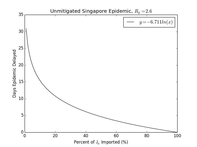
Graph 2.4– Plot of Days the Epidemic is Delayed against Imported Cases |
As can be seen, there is a vertical asymptote when no cases are imported, indicating that the epidemic will never start. If countries responded early enough to the outbreak by locking down their borders like North Korea had done, this may be the case. The effectiveness of the travel restriction rapidly decreases the less effective it is. According to this model, 99% effective travel restriction may delay the epidemic for up to 

According to a paper published in the journal Science, the shutdown of the Wuhan International Tianhe Airport on January 23rd, delayed the epidemic in the rest of China only by 3 to 5 days, and internationally up to 2 to 3 weeks until mid-February. According to their analysis of air traffic data there was an observed 86% reduction in the number of cases exported from China following this travel ban. According to my crude model, would correspond to a =13.2")
Limitations of this model
This model is based on the idealized scenario that all the imported cases would come in at the beginning of the epidemic on the first day, while in most cases in the real world, cases are imported over a period of time of days to weeks. Perhaps an interesting analysis is to look at how an COVID-19 epidemic has spread on a cruise ship such as the Diamond Princess. It is a closed population with a fixed number of initial infected cases, which is arguably the closest situation to the idealized scenario presented here.
Effect of “Government Lockdowns” (Movement Restrictions)
It is unrealistic to expect a government or its citizens to behave as if nothing has changed in an epidemic. We can see this from real world data, evidently, that most countries have not had their outbreaks infect more than 5% of their population, whereas in a previous section, it was predicted that around 80% to 90% of population will eventually become infected had the outbreak been unmitigated. This is due to drastic movement restrictions that have been implemented in most countries following an exponentially increasing number of cases.
I will investigate the hypothetical situation where following an uncontrolled outbreak, the Singaporean government implements a lockdown on a certain day after the beginning of the outbreak. What this means for the model is that the force of infection, , will be reduced by a certain percentage following the day of the lockdown. In the following Graph 3.1, I have plotted the unmitigated epidemic in solid lines, and a reduction of by 90% starting from day 91 and Day 101 respectively. (See code in Appendix E). As 

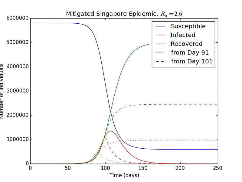 Graph 3.1– Initial Conditions: , , , Graph 3.1– Initial Conditions: , , ,  ; Reduction of 90% after lockdown on day 91 and 101: ; Reduction of 90% after lockdown on day 91 and 101:  , ,  |
As can be seen, the epidemic is essentially cut short starting from the day that the lockdown occurs, as the transmissibility of the virus is decreased drastically. Essentially, the red infected curve begins to exponentially decay as the sick recover at a rate of 
We can approximate this decay curve by looking back at the S-I-R differential equations:

")
Assuming 


=-\gamma t+c")


Substituting this into 


Obviously, 
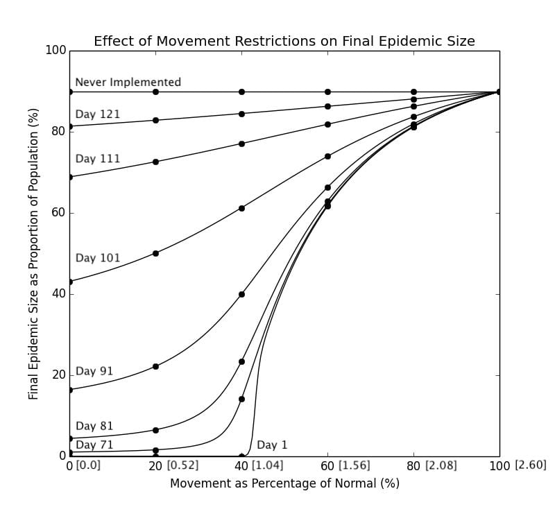 Graph 3.2– Final Epidemic Size as Proportion of Pop. Against Movement Restrictions; Numbers in Brackets[] along the x-axis are the corresponding R_0 |
As determined in a previous section, Day 107 is the peak of the number of current infected cases, so obviously, intervening after that would be ineffectual in significantly altering the course of the epidemic, as seen in the curves representing Day 111 and 121. In fact there is not a very significant difference as opposed to not intervening at all at this point, which will result in 89.9% of the population eventually becoming infected. The curves representing interventions on an earlier date are lower than that of curves representing intervening at a later date, and locking down even
It can be seen that reducing the $R_0$ by more than 60% is a significant value an effective lockdown measure, as 40% of 
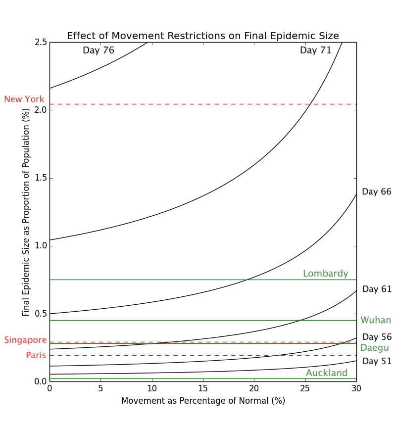 Graph 3.3– Epidemic Size of Cities as of May 1st, 2020 |
Obviously there is nowhere where cases have gotten as serious as to infect such a large proportion of the population. In Graph 3.3 above, I have plotted the corresponding percentages of the populations infected of some cities which have seen outbreaks of coronavirus.
Whilst the movement restriction model here is explicitly for Singapore, as all these cities have populations on the same order of magnitude, and changing these populations have very little impact on the trajectory of the epidemic, they can be compared with validity.
The cities marked in green have outbreaks that are largely over (Auckland, Daegu, Wuhan, and Lombardy), while the cities in red (Paris, Singapore, and New York) have outbreaks that are ongoing, and are thus likely to worsen. Again, using this simplistic model, it can be clearly seen here that delaying the lockdown by a few days could have a significant impact on the final number of COVID-19 cases. The difference between implementing a lockdown that decreases transmission to 0% on Day 76 and Day 71 may be the difference between having approximately 2.0% of the population infected v.s. 1.0% of the population. For example, Lombardy has 65% more cases per capita than Wuhan, but according to this model, this may be simply down to less than a 3-day difference in when their respective governments had implemented the lockdown.
From the graph, it can also be clearly seen that New York is experiencing a disproportionately severe outbreak as compared with most of the other cities. Based on this model, that may be either due to New York implementing the lockdown too late, having a lockdown that is not effective enough, or a combination of these two factors.
Limitations and Extensions
Obviously, the model only allows for relative comparison, as the number of days from the start of an outbreak is not absolute and will depend on when the epidemic has started in each country. Furthemore, it is difficult to define how much movement restrictions have reduced
When implementing social distancing and movement restrictions, it is also important for governments to take into account ethical and social concerns. These movement restrictions may disproportionately affect some groups of individuals, such as those who are homeless, disabled, unemployed, or have low income. The burden of workplace and school closure may result in both short and long term consequences for the livelihood and well-being of these people. It is important to further investigate the impact of social distancing measures to ensure that they are as equitable as they are effective.
Fitting the Model to Real World Data- New Zealand
In the following section, I will attempt to fit the above S-I-R model with a government movement restriction to the coronavirus epidemic in New Zealand. While I would like to use the Singapore data for this analysis as I have modelled Singapore for the previous portion of my investigation, the outbreak is still ongoing. Thus, it is still too early to see the tangible effect of the government “circuit breaker.” New Zealand has tested widely, provides transparent data, and has implemented a swift government lockdown and travel restrictions, so it is quite an ideal dataset (the data is from the European Center for Disease Control Global Dataset). I have changed nothing about the S-I-R model except to adjust the population size from 5.804 million to 4.815 million.
| New Zealand Population |  (2019) (2019) |
| Initial Force of Infection () |
|
| Rate of Recovery () |
|
| Days of Lockdown |  |
| Percent Reduction of |
90% |
New Zealand Model Key Characteristics
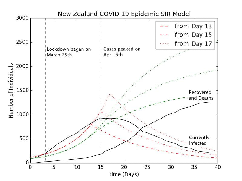
Graph 3.4– S-I-R Model of New Zealand Epidemic with Control Measures |
To allow for reasonable comparison of the New Zealand data with the S-I-R model, I have normalized everything to start from the day when the case count of the number of currently infected people surpassed
The set of curves representing a lockdown starting from Day 13 is perhaps the best fit for the New Zealand epidemic. The model predicts that just under 


However, there are several problems with the Day 13 model. New Zealand has already implemented a lockdown starting from March 25th, which is Day 3 in this model, and cases only peaked there on Day 15, a full 12 days after the lockdown had been implemented. According to the transmission dynamics of the S-I-R model, cases will peak immediately once the lockdown has been implemented due to the immediate reduction in the transmission rate. This discrepancy is probably due to a combination of factors. One may be the delay between when a person becomes infectious and when they are tested positive and thus recorded as a positive case. Perhaps the most important is the incubation period of the virus, of which the person is infected but is not infectious, in a stage which epidemiologists call “Exposed.” According to a study from the researchers at Johns Hopkins University, the incubation period ranges from 
Final Conclusions
In this investigation, I have explored several of the most important factors of the S-I-R compartmental model by implementing the differential equations in Python. Thus, I have been able to draw critical conclusions resulting from varying the following independent variables in the program. These are summarized below:
- Singapore S-I-R Model: Unmitigated epidemic may cause up to 89.9% of the population of 5.8 million becoming infected by COVID-19
- Effect of
- Effect of
- Effect of “Government Restrictions”: Time and strictness of implementation
- Fitting S-I-R Model with New Zealand Data
However, there are several limitations to this method of analysis. As the set of differential equations model continuous change, and the iterative program could only describe discrete change (albeit over many incremental time steps) there will always be a small discrepancy with the analytical solution. The S-I-R model itself is also quite simplistic in its assumptions:
- It assumes everyone in the population will have an equal probability from getting an infection from a diseased person. However, in reality, close contacts such as family members, peers, and colleagues are much more likely to be infected.
- Another unrealistic assumption is that people who are infected will immediately become infectious themselves. However, in reality, there is often an incubation period of several days the person becomes infectious. For COVID-19, as I have discussed, it averages to around 5 days. This is fairly significant considering that the infectious period is double that, around 10 days. A more advanced model, the S-E-I-R model, which has an extra “Exposed” category of individuals, takes that into account.
- The S-I-R model assumes that all parameters are constant and have no variance. In reality, there is often quite a wide variation of the infectious period and the recovery rate for each individual. Factors such as age and general health condition have been demonstrated in COVID-19 to have a large impact on these factors. Random stochastic variations resulting from this that may have a large bearing on the epidemic trajectory in the transmission rate are not factored into account.
- Quarantine and isolation measures reduce the effective infectious period of COVID-19. For example, a Cochrane meta-analysis indicated there is a significant benefit resulting from quarantining travelers to reduce imported cases and infected individuals to prevent further spread. The S-I-R model used here has not taken this into account.
Final Reflections
The COVID-19 pandemic is a current, ongoing event of drastic societal and personal significance to myself and the people around me. Through this exploration, I was not only able to gain a deeper understanding of the science and mathematics behind this, but also share some of this insight with my peers, enabling them to gain a deeper and perhaps more complete understanding of recent events. Whilst in the beginning I was perhaps overly ambitious about the scope of the project and spent a lot more time than I had anticipated especially going through the technical aspects of the Python programming, I was able to successfully overcome this challenge after many hours meticulously combing through the code and taking a basic online course on MatPlotLib.
In the past, my experience with science and mathematics projects have largely been groupwork, but this individual exploration taught me the importance of self-management and independent research. Meeting with my mentor, Mr. Mollitt and discussing my project with him was also a challenge to the remote nature of the discussions. However, due to the constraints on accessing physical media and materials from the lab as a result of COVID-19, I have developed skills that would be very useful for me in the future, such as finding and evaluating reliable online sources, analyzing large datasets, and computer programming.
This project introduced me to the world of computational epidemiology, and the close-knit interplay between statistics and healthcare. To further develop this project, I could apply this method of analysis to a larger number of countries to see whether it is as applicable as it is here. I could see extending this project into a possible educational tool to be used in classes as a way to teach students on mathematical topics such as calculus, logarithms, logistic and exponential growth, recursive relations, or in science classes in topics such as data analysis, epidemiology, and disease, all in relation to programming and computer science.
In the future, I would like to further investigate other models that could tackle some of the limitations as mentioned in the previous section and see how they are implemented with the assistance of a computer program.
Addendum: Parameter Estimation with Real-World Data
In this extra section, I will attempt to come up with estimates for the 2 key parameters,
Cumulative number of confirmed cases in the beginning:

Remaining Infectious Cases after Lockdown:
Estimating the Basic Reproductive Number,
In the graph below, I plot the cumulative number of cases since the day that total case count had surpassed
Graph 4.1 is a semilog plot of COVID-19 outbreaks in several countries compared with the theoretical exponential scenario as a straight line. As can be clearly seen, in the initial stages of the outbreak becoming uncontrolled and more widespread, the trend was clearly approximated by the exponential, indicating the
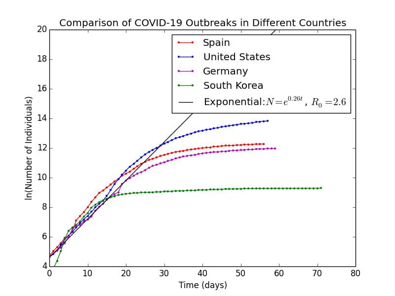 Graph 4.1– Semilog Plot of COVID-19 outbreaks in Spain, US, Germany, South Korea |
Graph 4.1 is a semilog plot of COVID-19 outbreaks in several countries compared with the theoretical exponential scenario as a straight line. As can be clearly seen, in the initial stages of the outbreak becoming uncontrolled and more widespread, the trend was clearly approximated by the exponential, indicating the
| Country | Data Taken up to Day | Calculated |
Correlation Coefficient ( ) ) |
| Spain | |
 |
 |
| United States | |
 |
 |
| Germany | |
 |
 |
| South Korea |  |
 |
 |
Obviously, epidemiologists have much more advanced models which they could use to calculate
Estimating the Duration of Disease, D
Here, we will use the data from three countries which have successfully controlled the outbreak: New Zealand, China, and Austria. As we have seen before, the remaining number of infections follows an exponential decay as described by the equation: 
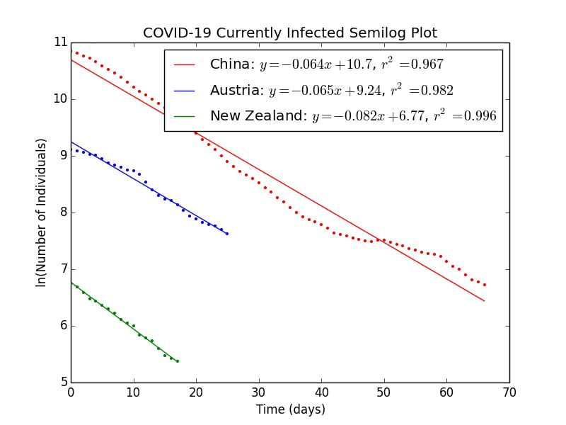 Graph 4.1– Semilog Plot of COVID-19 outbreaks in China, Austria, and New Zealand |
As can be seen in Graph 4.1, the remaining number of infectious cases in these countries decay in an exponential fashion as indicated by the linear relationships on a semilog scale. The correlation coefficients are close to
New Zealand example calculation
=ln(I_0)-\gamma t")


As


| Country | Rate of Recovery | Calculated |
Correlation Coefficient () |
| New Zealand |  |
 |
 |
| Austria |  |
|
 |
| China |  |
|
 |
The values of
References
Barbara Nussbaumer-Streit, Verena Mayr, Andreea Iulia Dobrescu, Andrea Chapman, Emma Persad, Irma Klerings, Gernot Wagner, Uwe Siebert, Claudia Christof, Casey Zachariah, Gerald Gartlehner. Quarantine alone or in combination with other public health measures to control COVID-19: a rapid review. Cochrane Database of Systematic Reviews, 2020; DOI: 10.1002/14651858.CD013574. Retrieved May 7th, 2020 from https://www.cochranelibrary.com/cdsr/doi/10.1002/14651858.CD013574/full
Biggerstaff, M., Cauchemez, S., Reed, C. et al. Estimates of the reproduction number for seasonal, pandemic, and zoonotic influenza: a systematic review of the literature. BMC Infectious Diseases 14, 480 (2014). Retrieved May 1st, 2020 from https://doi.org/10.1186/1471-2334-14-480
Centers for Disease Control and Prevention. Influenza (Flu). Retrieved May 1st, 2020 from https://www.cdc.gov/flu/index.htm
Chinazzi, Matteo, et al. “The Effect of Travel Restrictions on the Spread of the 2019 Novel Coronavirus (COVID-19) Outbreak.” Science, American Association for the Advancement of Science, 24 Apr. 2020, science.sciencemag.org/content/368/6489/395.full. DOI:10.1126/science.aba9757
David Smith and Lang Moore, “The SIR Model for Spread of Disease” Convergence (December 2004). Retrieved April 22nd, 2020 from https://www.maa.org/press/periodicals/loci/joma/the-sir-model-for-spread-of-disease-eulers-method-for-systems
European Center for Disease Control. (29th April 2020). COVID-19 Coronavirus data. DOI: 10.2906/101099100099/1. Retrieved April 30th, 2020 from https://www.ecdc.europa.eu/en/publications-data/download-todays-data-geographic-distribution-covid-19-cases-worldwide
Harko, T., Lobo, F. et al. (2014). Exact analytical solutions of the Susceptible-Infected-Recovered (S-I-R) epidemic model and of the S-I-R model with equal death and birth rates. Applied Mathematics and Computation. DOI:10.1016/j.amc.2014.03.030. Retrieved April 30th, 2020 from https://arxiv.org/abs/1403.2160
J. D. Hunter, “Matplotlib: A 2D Graphics Environment”, Computing in Science & Engineering, vol. 9, no. 3, pp. 90-95, 2007.
Joel R Koo, Alex R Cook, Minah Park, Yinxiaohe Sun, Haoyang Sun, Jue Tao Lim, Clarence Tam, Borame L Dickens. Interventions to mitigate early spread of SARS-CoV-2 in Singapore: a modelling study. The Lancet Infectious Diseases, 2020; DOI: 10.1016/S1473-3099(20)30162-6.
Joseph A Lewnard, Nathan C Lo. Scientific and ethical basis for social-distancing interventions against COVID-19. The Lancet Infectious Diseases, 2020; DOI: 10.1016/S1473-3099(20)30190-0. Retrieved May 17th from https://www.thelancet.com/pdfs/journals/laninf/PIIS1473-3099(20)30190-0.pdf
Lauer SA, Grantz KH, Bi Q, et al. The Incubation Period of Coronavirus Disease 2019 (COVID-19) From Publicly Reported Confirmed Cases: Estimation and Application. Ann Intern Med. 2020; [Epub ahead of print 10 March 2020]. DOI: https://doi.org/10.7326/M20-0504
MRC Centre for Global Infectious Disease Analysis. (3rd March, 2020). The Global Impact of COVID-19 and Strategies for Mitigation and Suppression. Retrieved April 28th from https://www.imperial.ac.uk/media/imperial-college/medicine/sph/ide/gida-fellowships/Imperial-College-COVID19-Global-Impact-26-03-2020v2.pdf
Magnus, Manya. Intermediate Epidemiology: Methods That Matter. Jones & Bartlett Learning, 2016.
Numberphile. (25th March, 2020). The Coronavirus Curve – Numberphile. Retrieved March 31st, 2020 from https://www.youtube.com/watch?v=k6nLfCbAzgo
Saw Swee Hock School of Public Health. (25th April, 2020). COVID-19 Science Report: Clinical Characteristics. Retrieved April 28th from https://sph.nus.edu.sg/wp-content/uploads/2020/04/COVID-19-Science-Report-Clinical-Characteristics-27-Apr.pdf
Weisstein, Eric W. “Kermack-McKendrick Model.” From MathWorld–A Wolfram Web Resource. https://mathworld.wolfram.com/Kermack-McKendrickModel.html
WHO The Global Health Observatory. (2020). Hospital beds (per 10 000 population). Retrieved May 1st from https://www.who.int/data/gho/data/indicators/indicator-details/GHO/hospital-beds-(per-10-000-population)
World Health Organization. (24th February, 2020). Report of the WHO-China Joint Mission on Coronavirus Disease 2019 (COVID-19). Retrieved April 28th, 2020 from https://www.who.int/docs/default-source/coronaviruse/who-china-joint-mission-on-covid-19-final-report.pdf
World Bank. (2018). Population Statistics 1960-2018. Retrieved from https://data.worldbank.org/indicator/SP.POP.TOTL
Van Rossum, G., & Drake Jr, F. L. (1995). Python reference manual. Centrum voor Wiskunde en Informatica Amsterdam.
Appendices
In the following Appendices, I have provided in full the most important pieces of code in the Python programming language that I have used over the course of the investigation. All the code here is original.
Appendix A- Code for SIR Singapore Epidemic
import cmath

import matplotlib.pyplot as plt

import numpy as np
S=5804000-1

I=1

R=0

R0=2.6

d=10.

a=R0/(S*d)

time=[0]

period=250

susceptible=[5804000-1]

infected=[1]

recovered=[0]

Trans=S*a

Recov=1/d
for t in range (1,period+1):
S=S-S*I*a

I=I+S*I*a-I/d

R=R+I/d

time.append(t)

susceptible.append(S)

infected.append(I)

recovered.append(R)
S=5804000

Proportion=100*(S-susceptible[period])/S

Peak=100*max(infected)/S
print "Transmission Rate=", Trans

print "Recovery Rate=", Recov

print "R0=", R0

print "Final Proportion Infected=", Proportion

print "Peak Proportion Infected=", Peak

print "Final Epidemic Size=", recovered[period]

print "time=", time

print "susceptible=", susceptible

print "infected=", infected

print "recovered=", recovered
plt.plot(time, susceptible, color='b', label='Susceptible')

plt.plot(time, infected, color='r', label='Infected')

plt.plot(time, recovered, color='g', label='Recovered')
plt.xlabel('Time (days)')

plt.ylabel('Number of Individuals')

plt.title('Unmitigated Singapore Epidemic, $R_0=2.6$')

plt.legend()

plt.show()
Appendix B-Code for Final Epidemic Size Against
from scipy import stats

import math

import numpy as np

import matplotlib.pyplot as plt
#Initial Conditions

R0=[0.0,0.2,0.4,0.6,0.8,1.0,1.2,1.4,1.6,1.8,2.0,2.2,2.4,2.6,2.8,3.0,3.2,3.4,3.6,3.8,4.0]

Final Epi Proportion=[]
for i in range (0, len(R0)):
S=5804000-1

I=1

R=0

d=10.

time=[0]

period=500

susceptible=[5804000-1]

infected=[1]

recovered=[0]

a=R0[i]/(S*d)

Trans=S*a

Recov=1/d

for t in range (1,period+1):
S=S-S*I*a

I=I+S*I*a-I/d

R=R+I/d

time.append(t)

susceptible.append(S)

infected.append(I)

recovered.append(R)
Proportion=100*(5804000-susceptible[period])/5804000

print Proportion

Peak=100*max(infected)/S

Finalepiproportion.append(Proportion)
plt.plot(R0, Finalepiproportion, 'ro', color='black')
#plot smooth line

R0cont=[]

Finalepiproportioncont=[]

for n in range (0,4000):

R0cont.append(0.001*n)

for i in range (0, len(R0cont)):

S=5804000-1

I=1

R=0

d=10.

time=[0]

period=500
susceptible=[5804000-1]

infected=[1]

recovered=[0]

a=R0cont[i]/(S*d)

Trans=S*a

Recov=1/d
for t in range (1,period+1):
S=S-S*I*a

I=I+S*I*a-I/d

R=R+I/d

time.append(t)

susceptible.append(S)

infected.append(I)

recovered.append(R)

Proportion=100*(5804000-susceptible[period])/5804000

print Proportion

Peak=100*max(infected)/S

Finalepiproportioncont.append(Proportion)
plt.plot(R0cont, Finalepiproportioncont, color='green')
plt.xlabel('Basic Reproductive Number ($R_0$)')

plt.ylabel('Final Epidemic Size as Proportion of Population (%)')

plt.title('Final Epidemic Size against $R_0$')

plt.legend()

plt.show()
Appendix C-Code for Peak Epidemic Size Against
from scipy import stats

import math

import numpy as np

import matplotlib.pyplot as plt
#Initial Conditions

R0=[0.0,0.2,0.4,0.6,0.8,1.0,1.28,1.4,1.6,1.8,2.0,2.2,2.4,2.6,2.8,3.0,3.2,3.4,3.6,3.8,4.0]

Peakepiproportion=[]
for i in range (0, len(R0)):
S=5804000-1

I=1

R=0

d=10.

time=[0]

period=500

susceptible=[5804000-1]

infected=[1]

recovered=[0]

a=R0[i]/(S*d)

Trans=S*a

Recov=1/d
for t in range (1,period+1):
S=S-S*I*a

I=I+S*I*a-I/d

R=R+I/d

time.append(t)

susceptible.append(S)

infected.append(I)

recovered.append(R)
Proportion=100*(5804000-susceptible[period])/5804000

Peak=100*max(infected)/5804000

Peakepiproportion.append(Peak)
plt.plot(R0, Peakepiproportion, 'ro', color='black')
#plot smooth line

R0cont=[]

Peakepiproportioncont=[]
for n in range (0,4000):
R0cont.append(0.001*n)
for i in range (0, len(R0cont)):
S=5804000-1

I=1

R=0

d=10.

time=[0]

period=500

susceptible=[5804000-1]

infected=[1]

recovered=[0]

a=R0cont[i]/(S*d)

Trans=S*a

Recov=1/d
for t in range (1,period+1):
S=S-S*I*a

I=I+S*I*a-I/d

R=R+I/d

time.append(t)

susceptible.append(S)

infected.append(I)

recovered.append(R)
Proportion=100*(5804000-susceptible[period])/5804000

Peak=100*max(infected)/5804000

Peakepiproportioncont.append(Peak)
plt.plot(R0cont, Peakepiproportioncont, color='black')
plt.xlabel('Basic Reproductive Number ($R_0$)')

plt.ylabel('Peak Epidemic Size as Proportion of Population (%)')

plt.title('Peak Epidemic Size against $R_0$')

plt.legend()

plt.show()
Appendix D- Code for Effect of Imported Cases on Singapore Epidemic
import cmath

import matplotlib.pyplot as plt

import numpy as np
#Initial Conditions

I=1

S=5804000-I

R=0

R0=2.6

d=10.

a=R0/(S*d)

time=[0]

period=250

susceptible=[5804000-I]

infected=[I]

recovered=[0]

Trans=S*a

Recov=1/d
for t in range (1,period+1):
S=S-S*I*a

I=I+S*I*a-I/d

R=R+I/d

time.append(t)

susceptible.append(S)

infected.append(I)

recovered.append(R)
S=5804000

Proportion=100*(S-susceptible[period])/S

Peak=100*max(infected)/S
print "Transmission Rate=", Trans

print "Recovery Rate=", Recov

print "R0=", R0

print "Final Proportion Infected=", Proportion

print "Peak Proportion Infected=", Peak

print "Final Epidemic Size=", recovered[period]
plt.plot(time, susceptible, color='b', label='Susceptible-1')

plt.plot(time, infected, color='r', label='Infected-1')

plt.plot(time, recovered, color='g', label='Recovered-1')
S=5804000-1000

I=1000

R=0

R0=2.6

d=10.

a=R0/(S*d)

time=[0]

period=250

susceptible=[5804000-1000]

infected=[1000]

recovered=[0]

Trans=S*a

Recov=1/d
for t in range (1,period+1):
S=S-S*I*a

I=I+S*I*a-I/d

R=R+I/d

time.append(t)

susceptible.append(S)

infected.append(I)

recovered.append(R)
plt.plot(time, susceptible, color='b', linestyle='dashed', label='Susceptible-1000')

plt.plot(time, infected, color='r', linestyle='dashed', label='Infected-1000')

plt.plot(time, recovered, color='g', linestyle='dashed', label='Recovered-1000')
plt.xlabel('Time (days)')

plt.ylabel('Number of Individuals')

plt.title('Unmitigated Singapore Epidemic, $R_0=2.6$')

plt.legend()

plt.show()
Appendix E- Code for Effect of Lockdown on Singapore Epidemic
from scipy import stats

import math

import matplotlib.pyplot as plt

import numpy as np
#Initial Conditions

S=5804000-1

I=1

R=0

R0=2.6

d=10.

a=R0/(S*d)

time=[0]

period=201

susceptible=[5804000-1]

infected=[1]

recovered=[0]

Trans=S*a

Recov=1/d

a=[0.26/S]

R0=S*a[0]*d
for t in range (1,201):
I=I+S*I*a[0]-I/d

S=S-S*I*a[0]

R=R+I/d

time.append(t)

susceptible.append(S)

infected.append(I)

recovered.append(R)
print "Transmission Rate=", Trans

print "Recovery Rate=", Recov

print "R0=", R0
plt.plot(time, susceptible, color='blue', label='Susceptible')

plt.plot(time, infected, color='red', label='Infected')

plt.plot(time, recovered, color='green', label='Recovered')
#Control Measures Applied on day lockd

lockd=[91,101]
for i in range (0,2):
S=5804000-1

I=1

R=0

a=[0.26/S,0.1*0.26/S]

d=10.

time=[0]

susceptible=[5804000-1]

infected=[1]

recovered=[0]
for t in range (1,lockd[i]):
I=I+S*I*a[0]-I/d

S=S-S*I*a[0]

R=R+I/d

time.append(t)

susceptible.append(S)

infected.append(I)

recovered.append(R)
for t in range (lockd[i],201):
I=I+S*I*a[1]-I/d

S=S-S*I*a[1]

R=R+I/d

time.append(t)

susceptible.append(S)

infected.append(I)

recovered.append(R)

x=lockd[i]
if i==0:
plt.plot(time, infected, ':', color='red', label='')

plt.plot(time, recovered, ':', color='green', label='')

plt.plot(time, susceptible, ':', color='blue', label='')

plt.plot(time, time, ':', color='black', label='from Day 91')
elif i==1:
plt.plot(time, infected, '--', color='red', label='')

plt.plot(time, recovered, '--', color='green', label='')

plt.plot(time, susceptible, '--', color='blue', label='')

plt.plot(time, time, '--', color='black', label='from Day 101')
plt.xlabel('Time (days)')

plt.ylabel('Number of Individuals')

plt.title('Mitigated Singapore Epidemic, $R_0=2.6$')

plt.legend()

plt.show()
Appendix F-Code for Effect of Lockdown on Singapore Epidemic
from scipy import stats

import math

import matplotlib.pyplot as plt

import numpy as np
Finalepiproportion=[]

FOIProp=[]

FOIPerc=[]
for n in range (0,201):
FOIProp.append(0.005*n)

FOIPerc.append(0.5*n)
for i in range (0,len(FOIProp)):
S=5804000.-1.

I=1.

R=0.

R0=2.6

d=10.

time=[0]

period=1000

susceptible=[5804000.-1]

infected=[1]

recovered=[0]

N=0

a=[0.26/S]

R0=S*a[0]*d
for t in range (1,period+1):
I=I+S*I*FOIProp[i]*a[0]-I/d

S=S-S*I*FOIProp[i]*a[0]

R=R+I/d

time.append(t)

susceptible.append(S)

infected.append(I)

recovered.append(R) Proportion=100*(5804000.-susceptible[period])/5804000.

Finalepiproportion.append(Proportion)

plt.plot(FOIPerc, Finalepiproportion, color='black')
for i in range (0,8):
Finalepiproportion=[]

lockd=[1,71,81,91,101,111,121,191]
for n in range (0, len(FOIProp)):
S=5804000.-1

I=1

R=0

a=[0.26/S,FOIProp[n]*0.26/S]

d=10.

time=[0]

susceptible=[5804000-1]

infected=[1]

recovered=[0]
for t in range (1,lockd[i]):
I=I+S*I*a[0]-I/d

S=S-S*I*a[0]

R=R+I/d

time.append(t)

susceptible.append(S)

infected.append(I)

recovered.append(R)
for t in range (lockd[i],period+1):
I=I+S*I*a[1]-I/d

S=S-S*I*a[1]

R=R+I/d

time.append(t)

susceptible.append(S)

infected.append(I)

recovered.append(R)

Proportion=100*(5804000-susceptible[period])/5804000

Finalepiproportion.append(Proportion)

plt.plot(FOIPerc, Finalepiproportion, color='black')
Finalepiproportion=[]

FOIProp=[]

FOIPerc=[]
for n in range (0,5):
FOIProp.append(0.2*n)

FOIPerc.append(20*n)
for i in range (0,8):
Finalepiproportion=[]

lockd=[1,71,81,91,101,111,121,191]
for n in range (0, len(FOIProp)):
S=5804000.-1

I=1

R=0

a=[0.26/S,FOIProp[n]*0.26/S]

d=10.

time=[0]

susceptible=[5804000-1]

infected=[1]

recovered=[0]
for t in range (1,lockd[i]):
I=I+S*I*a[0]-I/d

S=S-S*I*a[0]

R=R+I/d

time.append(t)

susceptible.append(S)

infected.append(I)

recovered.append(R)
for t in range (lockd[i],period+1):
I=I+S*I*a[1]-I/d

S=S-S*I*a[1]

R=R+I/d

time.append(t)

susceptible.append(S)

infected.append(I)

recovered.append(R)

Proportion=100*(5804000-susceptible[period])/5804000

Finalepiproportion.append(Proportion)

plt.plot(FOIPerc, Finalepiproportion, 'o', color='black')
plt.ylim((0,100))

Finalepiproportion=[]

FOIProp=[]

FOIPerc=[]
for n in range (0,5):
FOIProp.append(0.2*n)

FOIPerc.append(20*n)
for i in range (0,8):
Finalepiproportion=[]

lockd=[1,71,81,91,101,111,121,191]
for n in range (0, len(FOIProp)):
S=5804000.-1

I=1

R=0

a=[0.26/S,FOIProp[n]*0.26/S]

d=10.

time=[0]

susceptible=[5804000-1]

infected=[1]

recovered=[0]
for t in range (1,lockd[i]):
I=I+S*I*a[0]-I/d

S=S-S*I*a[0]

R=R+I/d

time.append(t)

susceptible.append(S)

infected.append(I)

recovered.append(R)
for t in range (lockd[i],period+1):
I=I+S*I*a[1]-I/d

S=S-S*I*a[1]

R=R+I/d

time.append(t)

susceptible.append(S)

infected.append(I)

recovered.append(R)

Proportion=100*(5804000-susceptible[period])/5804000

Finalepiproportion.append(Proportion)

print Finalepiproportion

plt.plot(FOIPerc, Finalepiproportion, 'o', color='black')
plt.ylim((0,100))

plt.xlabel('Movement as Percentage of Normal (%)')

plt.ylabel('Final Epidemic Size as Proportion of Population (%)')

plt.title('Effect of Movement Restrictions on Final Epidemic Size')

plt.legend()

plt.show()